00 Foundations
Linear and mass attenuation
μ = (μ/ρ) ρ. HVL = ln 2 / μ, TVL = ln 10 / μ.
Listen
Listen · English
Simulation
Linear and mass attenuation — Change the numbers; the scene follows.
Where it works
Water phantom
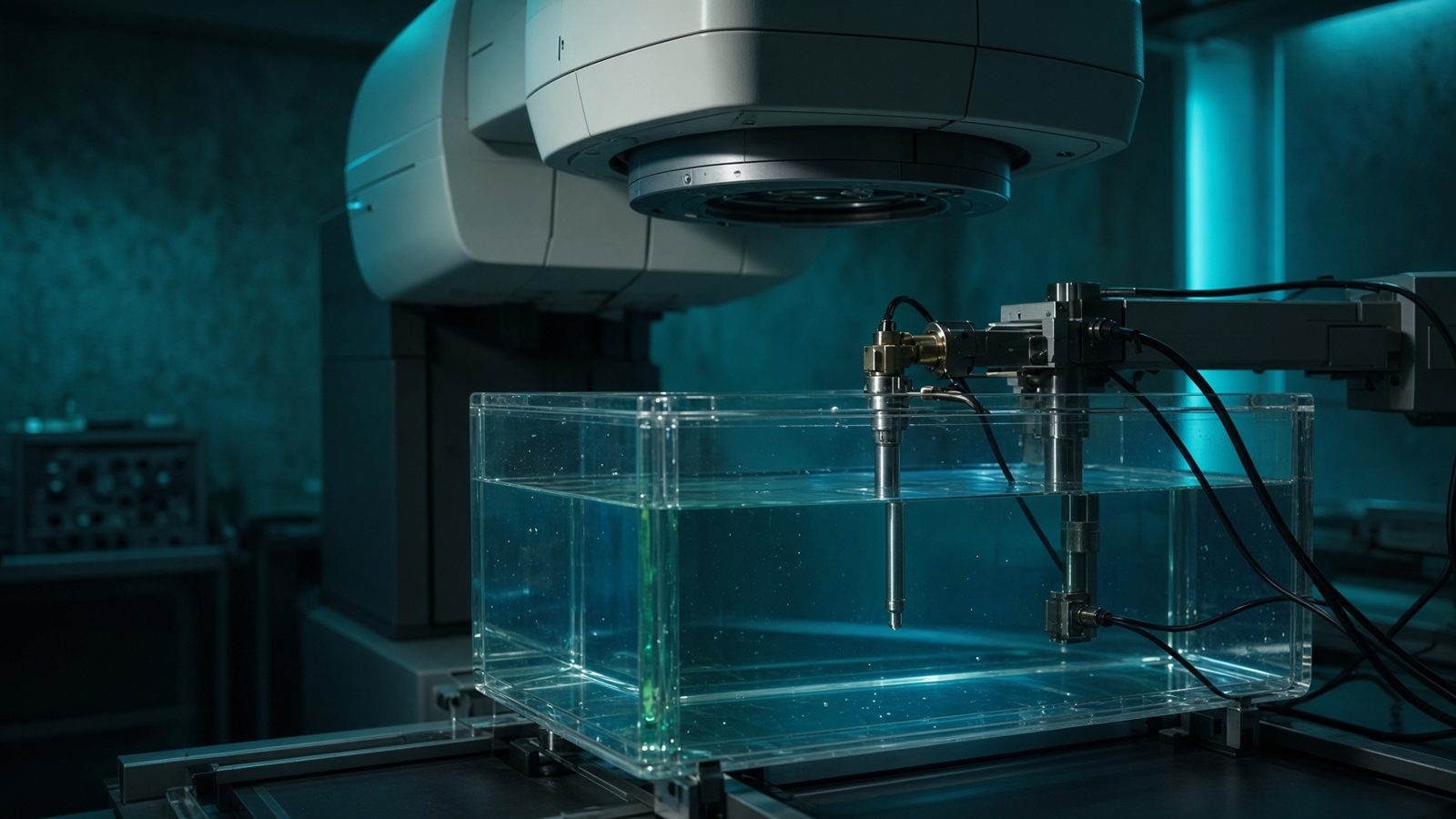
Ion chamber
In the water tank under the linac, at the ion chamber — reference dosimetry happens here.
Open this machineFormula
Variables
Results
μ
Linear coeff.
1.695cm⁻¹
HVL
Half-value layer
0.4089cm
TVL
Tenth-value layer
1.3585cm
I/I₀
Transmission
0.71248
Curve
Explanation
What it means
Mass attenuation μ/ρ is tabulated per element and energy (XCOM). Multiply by density to get the linear coefficient used in I = I₀ e^{−μx}. HVL is the thickness that halves a narrow beam; TVL reduces it by ten. For water at ~100 keV, μ/ρ ≈ 0.017 cm²/g so HVL ≈ 4 cm. This is a working relation in Radiation physics.
Where it is used
Clinically it sits on the Water phantom — Ion chamber. In the water tank under the linac, at the ion chamber — reference dosimetry happens here. Radiation physics lives at the x-ray target, the linac head, and inside the patient: how a photon is born, how it scatters, and how it dies. Use these relations before you trust a spectrum, a wall, or a kV-versus-MV contrast argument.
Water phantom · Open this machineHow to use it
Look up μ/ρ for your energy, enter density and thickness. The graph is narrow-beam transmission. Broad-beam shielding needs a buildup factor (see protection equations). Change one input and watch the curve and the simulation follow.
Symbols
- μ/ρMass attenuation0.15 cm²/g
- ρDensity11.3 g/cm³
- xThickness0.2 cm
Worked example
A typical case from the default values: μ/ρ = 0.15 cm²/g (Mass attenuation); ρ = 11.3 g/cm³ (Density); x = 0.2 cm (Thickness). Substituting into the relation gives μ = 1.695 cm⁻¹; HVL = 0.4089 cm; TVL = 1.3585 cm; I/I₀ = 0.71248. These are teaching numbers — align them with your machine.
Typical values give
- μ = 1.695cm⁻¹
- HVL = 0.4089cm
- TVL = 1.3585cm
- I/I₀ = 0.71248
Where it comes from
The displayed formula is the working relation. μ = (μ/ρ) ρ. HVL = ln 2 / μ, TVL = ln 10 / μ. Usual reference: NIST XCOM / Attix. Derive it in the specialty lesson, then return here to pin the numbers.
Reference: NIST XCOM / Attix
Assumptions & limits
Narrow-beam, good geometry: no scatter reaching the detector. Buildup, polychromatic beams (beam hardening), and K-edge structure are not in this calculator.
Pitfalls
Do not mix free-electron Compton kinematics with photoelectric-dominated kV imaging. Check keV versus MeV, and never treat a spectrum as one photon. Narrow-beam, good geometry: no scatter reaching the detector. Buildup, polychromatic beams (beam hardening), and K-edge structure are not in this calculator.
Keep this
Photons do not deposit dose; the electrons they set in motion do. Narrow-beam, good geometry: no scatter reaching the detector. Buildup, polychromatic beams (beam hardening), and K-edge structure are not in this calculator.
In this specialty