00 Foundations

Average LET from energy and range

Track-averaged LET ≈ E / R. Unrestricted collisional stopping power.

Play lecture Cast to TV

Listen

Listen · English

Simulation

Average LET from energy and range — Change the numbers; the scene follows.

Where it works

Proton gantry

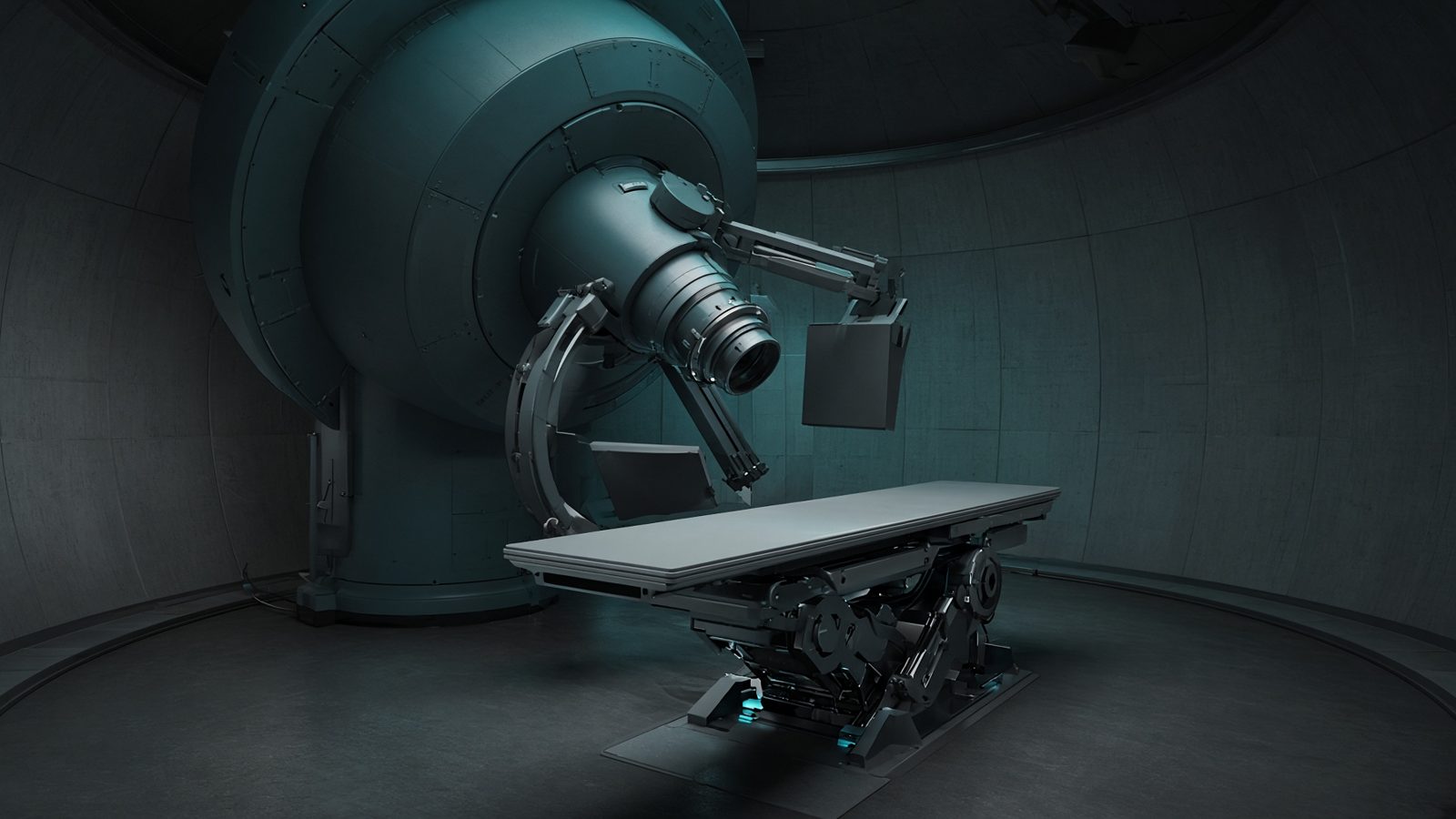
Patient / Bragg peak

Along the proton path in tissue, from the snout to the distal Bragg peak.

Open this machine

Formula

\overline{L}_\infty \approx \frac{E}{R} = \left\langle\frac{dE}{dx}\right\rangle_{\mathrm{track}}

Typical values

Variables

E · Kinetic energyMeVR · Rangecm

Results

L̄
Track-average LET
0.7692keV/μm
S
Stopping power
7.6923MeV/cm
S/ρ
Mass stopping power
7.6923MeV·cm²/g

Explanation

\overline{L}_\infty \approx \frac{E}{R} = \left\langle\frac{dE}{dx}\right\rangle_{\mathrm{track}}

What it means

Linear energy transfer is the energy locally imparted per unit track length. Dividing the particle’s kinetic energy by its CSDA range gives the track-averaged unrestricted LET — a useful order-of-magnitude number. 6 MV electrons (E≈2 MeV, R≈1 cm) sit near 0.2 keV/μm (low LET); a 5 MeV α in water (R≈0.04 mm) is ~100 keV/μm (high LET, RBE ≫ 1). This is a working relation in Radiation physics.

Where it is used

Clinically it sits on the Proton gantry — Patient / Bragg peak. Along the proton path in tissue, from the snout to the distal Bragg peak. Radiation physics lives at the x-ray target, the linac head, and inside the patient: how a photon is born, how it scatters, and how it dies. Use these relations before you trust a spectrum, a wall, or a kV-versus-MV contrast argument.

Proton gantry · Open this machine

How to use it

Enter kinetic energy (MeV) and range (cm). The calculator reports keV/μm, MeV/cm and MeV·cm²/g for ρ = 1 g/cm³. Compare protons at mid-SOBP (~2–5 keV/μm) with carbon ions (~30–80 keV/μm). Change one input and watch the curve and the simulation follow.

Symbols

EKinetic energy200 MeV
RRange26 cm

Worked example

A typical case from the default values: E = 200 MeV (Kinetic energy); R = 26 cm (Range). Substituting into the relation gives L̄ = 0.7692 keV/μm; S = 7.6923 MeV/cm; S/ρ = 7.6923 MeV·cm²/g. These are teaching numbers — align them with your machine.

Typical values give

L̄ = 0.7692keV/μm
S = 7.6923MeV/cm
S/ρ = 7.6923MeV·cm²/g

Where it comes from

The displayed formula is the working relation. Track-averaged LET ≈ E / R. Unrestricted collisional stopping power. Usual reference: ICRU 85 / Hall. Derive it in the specialty lesson, then return here to pin the numbers.

Reference: ICRU 85 / Hall

Assumptions & limits

Track average, not dose average (z_D). Unrestricted (Δ=∞); restricted LET excludes δ-rays above a cutoff. Nuclear interactions and straggling ignored. For ions use a TPS or ICRU tables.

Pitfalls

Do not mix free-electron Compton kinematics with photoelectric-dominated kV imaging. Check keV versus MeV, and never treat a spectrum as one photon. Track average, not dose average (z_D). Unrestricted (Δ=∞); restricted LET excludes δ-rays above a cutoff. Nuclear interactions and straggling ignored. For ions use a TPS or ICRU tables.

Keep this

Photons do not deposit dose; the electrons they set in motion do. Track average, not dose average (z_D). Unrestricted (Δ=∞); restricted LET excludes δ-rays above a cutoff. Nuclear interactions and straggling ignored. For ions use a TPS or ICRU tables.

In this specialty

Radiation physics