00 Foundations

Klein–Nishina cross section

Unpolarised Compton differential cross section per electron versus scatter angle.

Play lecture Cast to TV

Listen

Listen · English

Simulation

Klein–Nishina cross section — Change the numbers; the scene follows.

Where it works

Linear accelerator

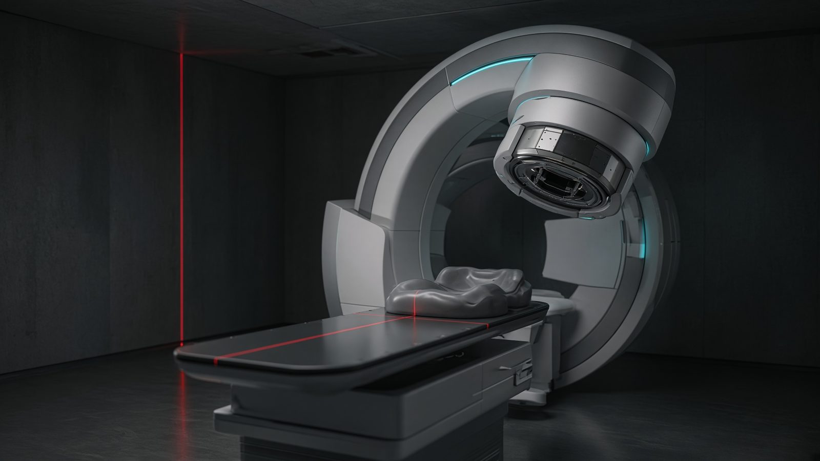
Isocenter

At isocenter, on the central axis through the patient (or a phantom in the same place).

Open this machine

Formula

\frac{d\sigma}{d\Omega}=\frac{r_e^2}{2}\left(\frac{E'}{E}\right)^2\left(\frac{E'}{E}+\frac{E}{E'}-\sin^2\theta\right)

Variables

E · Photon energykeVθ · Scatter angle°

Results

dσ/dΩ
Differential cross section
0.0287b/sr
E′/E
Kinematic ratio
0.8363
E′
Scattered energy
83.6334keV

Curve

Explanation

\frac{d\sigma}{d\Omega}=\frac{r_e^2}{2}\left(\frac{E'}{E}\right)^2\left(\frac{E'}{E}+\frac{E}{E'}-\sin^2\theta\right)

What it means

Klein–Nishina is the quantum-electrodynamic cross section for Compton scatter from a free electron. At diagnostic energies (~30–150 keV) scatter is almost isotropic in the forward half; at MV and PET energies it is strongly forward-peaked. Integrating over angle gives the Compton attenuation coefficient τ_C = Z n_e σ_KN. This is a working relation in Radiation physics.

Where it is used

Clinically it sits on the Linear accelerator — Isocenter. At isocenter, on the central axis through the patient (or a phantom in the same place). Radiation physics lives at the x-ray target, the linac head, and inside the patient: how a photon is born, how it scatters, and how it dies. Use these relations before you trust a spectrum, a wall, or a kV-versus-MV contrast argument.

Linear accelerator · Open this machine

How to use it

Enter incident photon energy E (keV) and scatter angle θ. Read dσ/dΩ in barn/sr and the Compton kinematic factor E′/E. Use it when teaching why anti-scatter grids and PET collimation work, and why MV scatter is a small-angle problem. Change one input and watch the curve and the simulation follow.

Symbols

EPhoton energy100 keV
θScatter angle90 °

Worked example

100 keV at 90°: E′/E ≈ 0.836, dσ/dΩ ≈ 0.041 barn/sr — about half the Thomson value r_e²/2. In numbers: E = 100 keV (Photon energy); θ = 90 ° (Scatter angle) → dσ/dΩ = 0.0287 b/sr; E′/E = 0.8363; E′ = 83.6334 keV.

Typical values give

dσ/dΩ = 0.0287b/sr
E′/E = 0.8363
E′ = 83.6334keV

Where it comes from

Start from the QED amplitude for γe → γe. The kinematic factor E′/E = 1 / [1 + (E/mc²)(1−cos θ)] multiplies the classical Thomson angular term (1+cos²θ)/2 after the Klein–Nishina correction (E′/E + E/E′ − sin²θ).

Reference: Klein & Nishina 1929 / Attix

Assumptions & limits

Free electron at rest; no binding, no Doppler broadening, no polarisation. Coherent (Rayleigh) scatter dominates at very low E and high Z and is not included. r_e = 2.818 fm.

Pitfalls

Do not mix free-electron Compton kinematics with photoelectric-dominated kV imaging. Check keV versus MeV, and never treat a spectrum as one photon. Free electron at rest; no binding, no Doppler broadening, no polarisation. Coherent (Rayleigh) scatter dominates at very low E and high Z and is not included. r_e = 2.818 fm.

Keep this

Photons do not deposit dose; the electrons they set in motion do. Free electron at rest; no binding, no Doppler broadening, no polarisation. Coherent (Rayleigh) scatter dominates at very low E and high Z and is not included. r_e = 2.818 fm.

In this specialty

Radiation physics