07 MRI
Slice thickness from gradient
Δz = BW_rf / (γ G_ss). Thinner slices need more gradient or less RF bandwidth.
Listen
Listen · English
Simulation
Slice thickness from gradient — Change the numbers; the scene follows.
Where it works
MRI scanner
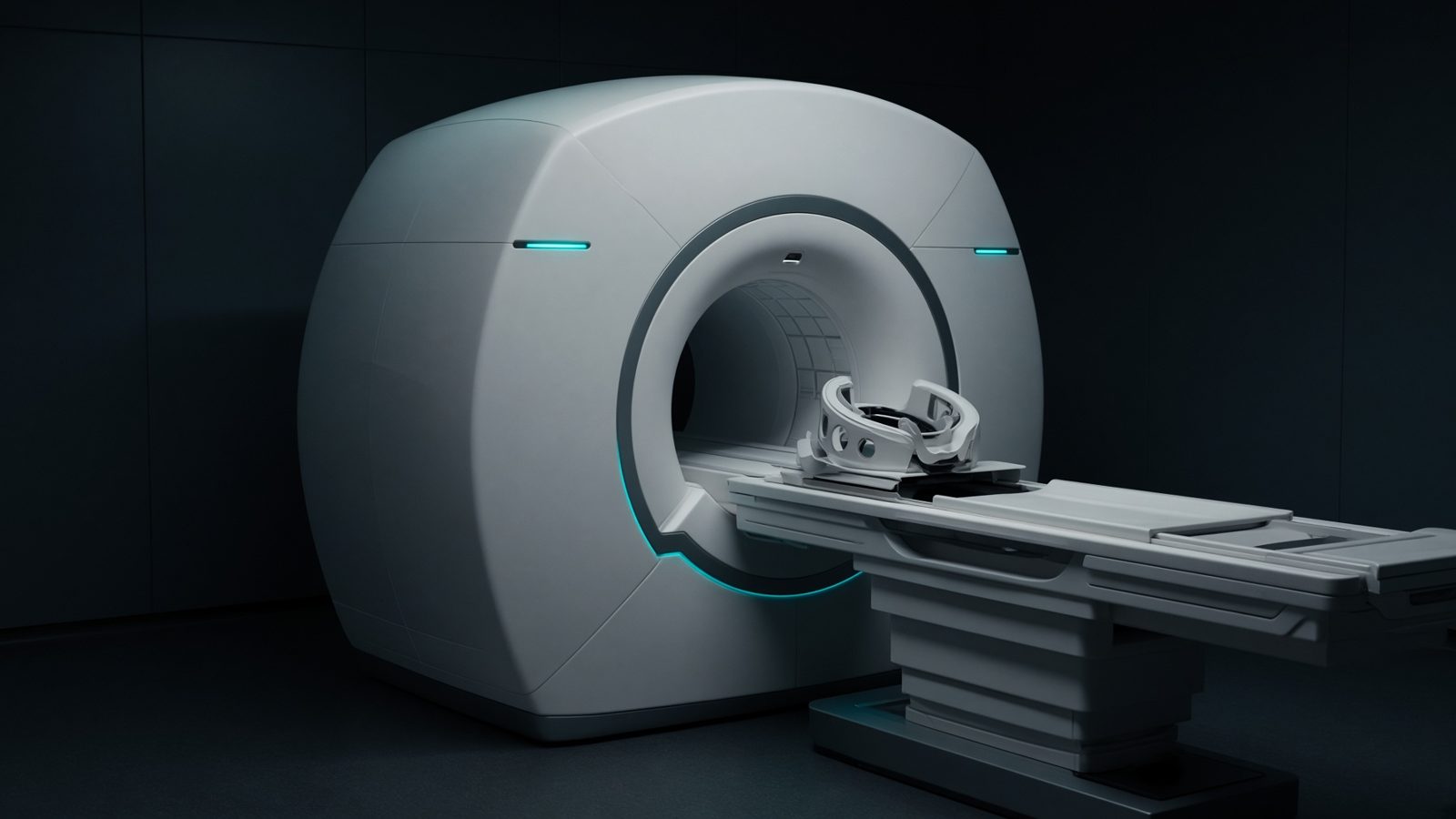
Gradient coils
In the gradient coils — slice thickness, FOV, diffusion encoding, voxel size.
Open this machineFormula
Variables
Results
Δz
Slice thickness
2.3487mm
Δz
Slice thickness
0.2349cm
Explanation
What it means
Slice thickness is RF bandwidth divided by the slice-select gradient (in Hz per metre). Steeper G_ss or narrower RF pulses give thinner slices, at the cost of more eddy currents / heating and a longer pulse. This is a working relation in MRI physics.
Where it is used
Clinically it sits on the MRI scanner — Gradient coils. In the gradient coils — slice thickness, FOV, diffusion encoding, voxel size. MRI physics lives in the magnet, the gradient, and the voxel: Larmor, Ernst, diffusion, and SAR. These relations decide whether a sequence is possible, safe, and worth the time.
MRI scanner · Open this machineHow to use it
γ/2π for ¹H is 42.577 MHz/T. 1000 Hz RF on 10 mT/m → Δz = 2.3 mm. Multi-slice gaps are extra (you still need space for imperfect profiles). Change one input and watch the curve and the simulation follow.
Symbols
- BWRF pulse bandwidth1,000 Hz
- G_ssSlice-select gradient10 mT/m
- γ/2πGyromagnetic ratio42.577 MHz/T
Worked example
A typical case from the default values: BW = 1,000 Hz (RF pulse bandwidth); G_ss = 10 mT/m (Slice-select gradient); γ/2π = 42.577 MHz/T (Gyromagnetic ratio). Substituting into the relation gives Δz = 2.3487 mm; Δz = 0.2349 cm. These are teaching numbers — align them with your machine.
Typical values give
- Δz = 2.3487mm
- Δz = 0.2349cm
Where it comes from
The displayed formula is the working relation. Δz = BW_rf / (γ G_ss). Thinner slices need more gradient or less RF bandwidth. Usual reference: McRobbie / Hashemi. Derive it in the specialty lesson, then return here to pin the numbers.
Reference: McRobbie / Hashemi
Assumptions & limits
Rectangular (sinc) profile idealisation. Real pulses have side lobes; the ‘nominal’ thickness is FWHM of the profile. Chemical shift also displaces fat slices.
Pitfalls
γ for ¹H is not γ for ¹³C. Ernst angle needs the true T1 at that field, not a 1.5 T table used at 3 T. SAR scales with B₀² and flip² — a 3 T copy of a 1.5 T protocol is not automatically legal. Rectangular (sinc) profile idealisation. Real pulses have side lobes; the ‘nominal’ thickness is FWHM of the profile. Chemical shift also displaces fat slices.
Keep this
Name the nucleus and the field before you quote a Larmor frequency. Rectangular (sinc) profile idealisation. Real pulses have side lobes; the ‘nominal’ thickness is FWHM of the profile. Chemical shift also displaces fat slices.
In this specialty