07 MRI
Apparent diffusion coefficient
S = S₀ e^{−b ADC} ⇒ ADC = ln(S₀/S) / b.
Listen
Listen · English
Simulation
Apparent diffusion coefficient — Change the numbers; the scene follows.
Where it works
MRI scanner
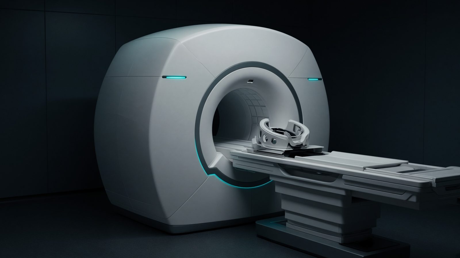
Patient in bore
In the tissue inside the bore — relaxation, fat/water, contrast, flow, magic angle.
Open this machineFormula
Variables
Results
ADC
Apparent diffusion coefficient
0.5978×10⁻³ mm²/s
ADC
ADC
0.000598mm²/s
Curve
Explanation
What it means
In a mono-exponential model the signal falls as e^{−b ADC}. Free water at 37 °C is ~3×10⁻³ mm²/s; grey matter ~0.8, white matter (along fibres) ~1.0, restricted tumour / cytotoxic oedema ~0.4–0.6, cysts ~3. Two-point ADC from b=0 and b=1000 is what most PACS show; a 3-point fit (0, 500, 1000) reduces perfusion contamination of the b=0 image (IVIM). This is a working relation in MRI physics.
Where it is used
Clinically it sits on the MRI scanner — Patient in bore. In the tissue inside the bore — relaxation, fat/water, contrast, flow, magic angle. MRI physics lives in the magnet, the gradient, and the voxel: Larmor, Ernst, diffusion, and SAR. These relations decide whether a sequence is possible, safe, and worth the time.
MRI scanner · Open this machineHow to use it
Enter S₀, S and b (s/mm²). Read ADC in 10⁻³ mm²/s. A 55% residual signal at b=1000 → ADC = 0.60 × 10⁻³ mm²/s (restricted). Change one input and watch the curve and the simulation follow.
Symbols
- S_0b=0 signal1,000
- SDiffusion-weighted signal550
- bb-value1,000 s/mm²
Worked example
A typical case from the default values: S_0 = 1,000 (b=0 signal); S = 550 (Diffusion-weighted signal); b = 1,000 s/mm² (b-value). Substituting into the relation gives ADC = 0.5978 ×10⁻³ mm²/s; ADC = 0.000598 mm²/s. These are teaching numbers — align them with your machine.
Typical values give
- ADC = 0.5978×10⁻³ mm²/s
- ADC = 0.000598mm²/s
Where it comes from
The displayed formula is the working relation. S = S₀ e^{−b ADC} ⇒ ADC = ln(S₀/S) / b. Usual reference: Le Bihan / McRobbie. Derive it in the specialty lesson, then return here to pin the numbers.
Reference: Le Bihan / McRobbie
Assumptions & limits
Mono-exponential, isotropic. IVIM, kurtosis and fibre anisotropy all deviate. S₀ must be the b=0 (or low-b) image of the same series, not a T2 FSE.
Pitfalls
γ for ¹H is not γ for ¹³C. Ernst angle needs the true T1 at that field, not a 1.5 T table used at 3 T. SAR scales with B₀² and flip² — a 3 T copy of a 1.5 T protocol is not automatically legal. Mono-exponential, isotropic. IVIM, kurtosis and fibre anisotropy all deviate. S₀ must be the b=0 (or low-b) image of the same series, not a T2 FSE.
Keep this
Name the nucleus and the field before you quote a Larmor frequency. Mono-exponential, isotropic. IVIM, kurtosis and fibre anisotropy all deviate. S₀ must be the b=0 (or low-b) image of the same series, not a T2 FSE.
In this specialty