07 MRI
Diffusion b-value
b = (γ G δ)² (Δ − δ/3) for a pair of rectangular pulses (Stejskal–Tanner).
Listen
Listen · English
Simulation
Diffusion b-value — Change the numbers; the scene follows.
Where it works
MRI scanner
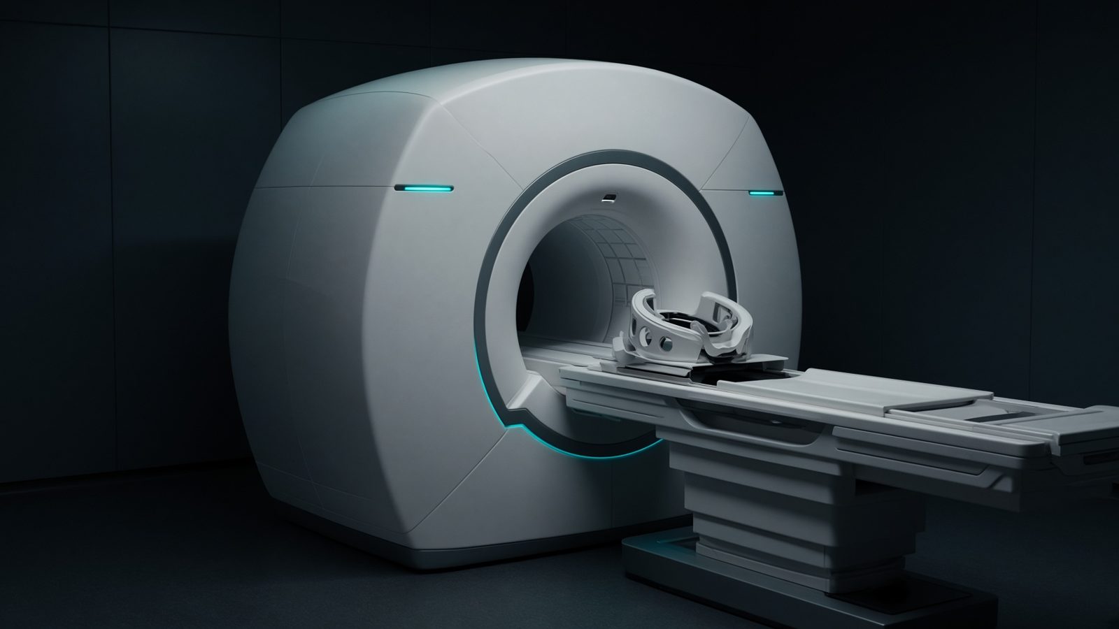
Gradient coils
In the gradient coils — slice thickness, FOV, diffusion encoding, voxel size.
Open this machineFormula
Variables
Results
b
b-value
858.8174s/mm²
Δ−δ/3
Effective diffusion time
33.3333ms
Explanation
What it means
The b-value is the diffusion-weighting dose: how hard the sequence punishes moving spins. Two matched gradient lobes around the 180° (spin-echo) or of opposite sign (STEAM) give b ∝ G² δ² (Δ − δ/3). Clinical DWI uses b = 0 and b = 800–1000 s/mm²; oncology and body DWI go to 1500–2000. ADC maps are a fit of ln S versus b. This is a working relation in MRI physics.
Where it is used
Clinically it sits on the MRI scanner — Gradient coils. In the gradient coils — slice thickness, FOV, diffusion encoding, voxel size. MRI physics lives in the magnet, the gradient, and the voxel: Larmor, Ernst, diffusion, and SAR. These relations decide whether a sequence is possible, safe, and worth the time.
MRI scanner · Open this machineHow to use it
Enter G (mT/m), lobe duration δ (ms) and spacing Δ (ms). γ for ¹H is built in (42.58 MHz/T = 2.675×10⁸ rad/s/T). 30 mT/m, δ = 20 ms, Δ = 40 ms → b ≈ 850 s/mm². Change one input and watch the curve and the simulation follow.
Symbols
- GGradient amplitude30 mT/m
- δLobe duration20 ms
- ΔLobe spacing40 ms
Worked example
A typical case from the default values: G = 30 mT/m (Gradient amplitude); δ = 20 ms (Lobe duration); Δ = 40 ms (Lobe spacing). Substituting into the relation gives b = 858.8174 s/mm²; Δ−δ/3 = 33.3333 ms. These are teaching numbers — align them with your machine.
Typical values give
- b = 858.8174s/mm²
- Δ−δ/3 = 33.3333ms
Where it comes from
The displayed formula is the working relation. b = (γ G δ)² (Δ − δ/3) for a pair of rectangular pulses (Stejskal–Tanner). Usual reference: Stejskal & Tanner 1965 / McRobbie. Derive it in the specialty lesson, then return here to pin the numbers.
Reference: Stejskal & Tanner 1965 / McRobbie
Assumptions & limits
Rectangular lobes, no ramp time, no imaging gradients. Real EPI-DWI b-matrices include the readout train and are 3×3 tensors (anisotropy). Cross-terms appear when you combine axes.
Pitfalls
γ for ¹H is not γ for ¹³C. Ernst angle needs the true T1 at that field, not a 1.5 T table used at 3 T. SAR scales with B₀² and flip² — a 3 T copy of a 1.5 T protocol is not automatically legal. Rectangular lobes, no ramp time, no imaging gradients. Real EPI-DWI b-matrices include the readout train and are 3×3 tensors (anisotropy). Cross-terms appear when you combine axes.
Keep this
Name the nucleus and the field before you quote a Larmor frequency. Rectangular lobes, no ramp time, no imaging gradients. Real EPI-DWI b-matrices include the readout train and are 3×3 tensors (anisotropy). Cross-terms appear when you combine axes.
In this specialty