02 Imaging
Bucky factor from transmission
B = (primary + scatter in) / (primary + scatter out of the grid).
Listen
Listen · English
Simulation
Bucky factor from transmission — Change the numbers; the scene follows.
Where it works
Radiography room
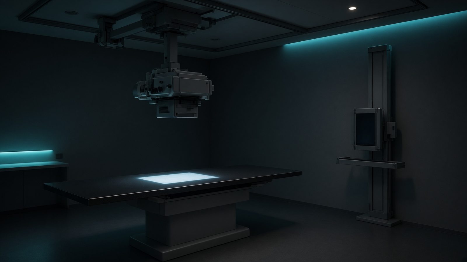
Bucky / detector
In the Bucky / detector: grid, AEC, DQE, and the pixel that samples the image.
Open this machineFormula
Variables
Results
B
Bucky factor
3.4884
SPR_in
Scatter-to-primary in
2
SPR_out
Scatter-to-primary out
0.2286
Explanation
What it means
The Bucky factor is how much you must raise mAs when inserting a grid: incident (primary+scatter) over what the grid transmits. It also yields scatter-to-primary ratios before and after the grid. This is a working relation in Diagnostic imaging.
Where it is used
Clinically it sits on the Radiography room — Bucky / detector. In the Bucky / detector: grid, AEC, DQE, and the pixel that samples the image. Diagnostic equations live on the tube, the detector, and the patient: magnification, air kerma, CTDI, and why bone lights up at 70 kV. They turn a technique chart into physics you can defend.
Radiography room · Open this machineHow to use it
Estimate I_s/I_p from thickness and kVp (SPR often 2–5 in abdomen). A good grid might pass 70% of primary and 8% of scatter → B ≈ 4. Change one input and watch the curve and the simulation follow.
Symbols
- I_pIncident primary100 a.u.
- I_sIncident scatter200 a.u.
- T_pPrimary transmission0.7
- T_sScatter transmission0.08
Worked example
A typical case from the default values: I_p = 100 a.u. (Incident primary); I_s = 200 a.u. (Incident scatter); T_p = 0.7 (Primary transmission); T_s = 0.08 (Scatter transmission). Substituting into the relation gives B = 3.4884; SPR_in = 2; SPR_out = 0.2286. These are teaching numbers — align them with your machine.
Typical values give
- B = 3.4884
- SPR_in = 2
- SPR_out = 0.2286
Where it comes from
The displayed formula is the working relation. B = (primary + scatter in) / (primary + scatter out of the grid). Usual reference: Bushberg. Derive it in the specialty lesson, then return here to pin the numbers.
Reference: Bushberg
Assumptions & limits
Simple two-channel model. Real grids have finite selectivity, focus distance, and K-factor (contrast improvement) that this calculator does not output separately.
Pitfalls
kVp is not the same as effective energy. CTDI is not patient dose — SSDE and organ dose come after. Do not quote DLP as if it were effective dose without a k-factor. Simple two-channel model. Real grids have finite selectivity, focus distance, and K-factor (contrast improvement) that this calculator does not output separately.
Keep this
Technique is physics: kV sets contrast, mAs sets noise, filtration sets the spectrum. Simple two-channel model. Real grids have finite selectivity, focus distance, and K-factor (contrast improvement) that this calculator does not output separately.
In this specialty