05 Biology
LQ-linear (high dose per fraction)
LQ is applied only up to D_t = 2 α/β; beyond that the survival curve is linear with slope γ = α + 2 β D_t.
Listen
Listen · English
Simulation
LQ-linear (high dose per fraction) — Change the numbers; the scene follows.
Where it works
Linear accelerator
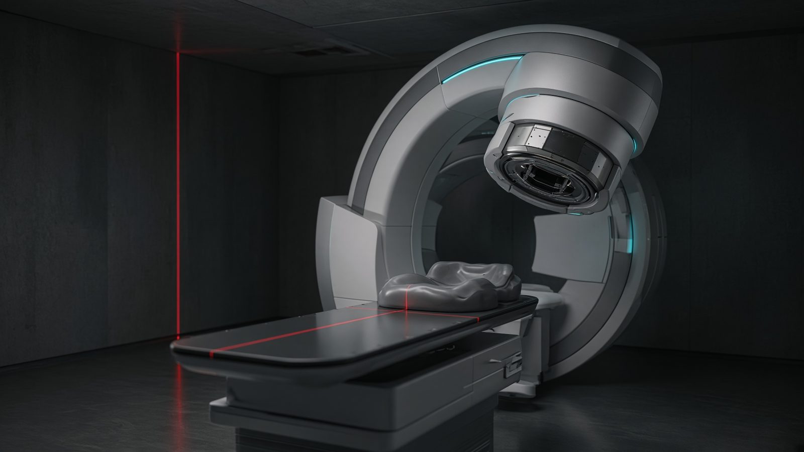
Isocenter
In the treated volume — tumour and OARs at isocenter, after the dose has been delivered.
Open this machineFormula
Variables
Results
D_t
Transition dose
20Gy
−ln S
LQ-L
6
−ln S_LQ
Pure LQ
6
ratio
LQ / LQ-L
1
Explanation
What it means
LQ overestimates cell kill (and BED) at the large doses per fraction of SBRT because the log-survival curve is seen to straighten. LQ-L (or USC, universal survival curve) keeps LQ up to a transition dose D_t ≈ 2 α/β and then a linear tangent. For α/β = 10 Gy, D_t ≈ 20 Gy so a 18 Gy × 3 SBRT scheme is only mildly affected; for α/β = 3 Gy, D_t ≈ 6 Gy and a 10 Gy fraction is well into the linear region. This is a working relation in Radiobiology.
Where it is used
Clinically it sits on the Linear accelerator — Isocenter. In the treated volume — tumour and OARs at isocenter, after the dose has been delivered. Radiobiology sits between the prescription and the organ-at-risk: LQ, BED, EQD2, and why 2 Gy is not 2 Gy if the fraction size changed. Use it to compare regimens, not to invent one.
Linear accelerator · Open this machineHow to use it
Enter α, β, dose per fraction D and optionally D_t (defaults to 2 α/β). Read −ln S, the pure-LQ value, and the ratio. Use it as a sanity check on BED for d > 8 Gy. Change one input and watch the curve and the simulation follow.
Symbols
- αAlpha0.3 Gy⁻¹
- βBeta0.03 Gy⁻²
- DDose per fraction10 Gy
- D_tTransition (0 = 2α/β)0 Gy
Worked example
A typical case from the default values: α = 0.3 Gy⁻¹ (Alpha); β = 0.03 Gy⁻² (Beta); D = 10 Gy (Dose per fraction); D_t = 0 Gy (Transition (0 = 2α/β)). Substituting into the relation gives D_t = 20 Gy; −ln S = 6; −ln S_LQ = 6; ratio = 1. These are teaching numbers — align them with your machine.
Typical values give
- D_t = 20Gy
- −ln S = 6
- −ln S_LQ = 6
- ratio = 1
Where it comes from
The displayed formula is the working relation. LQ is applied only up to D_t = 2 α/β; beyond that the survival curve is linear with slope γ = α + 2 β D_t. Usual reference: Astrahan / Guerrero & Li / Joiner. Derive it in the specialty lesson, then return here to pin the numbers.
Reference: Astrahan / Guerrero & Li / Joiner
Assumptions & limits
One of several high-dose recipes (USC, MKM, G-function). Transition dose is not a measured universal. Does not include reoxygenation, which may dominate SBRT biology more than the shape of SF.
Pitfalls
α/β is a model parameter, not a measured organ. BED from incomplete repair or a changed overall time is not the simple n·d·(1+d/(α/β)). Never EQD2 a stereotactic dose with an α/β you did not state. One of several high-dose recipes (USC, MKM, G-function). Transition dose is not a measured universal. Does not include reoxygenation, which may dominate SBRT biology more than the shape of SF.
Keep this
Always write α/β and the fraction size next to a BED or EQD2. One of several high-dose recipes (USC, MKM, G-function). Transition dose is not a measured universal. Does not include reoxygenation, which may dominate SBRT biology more than the shape of SF.
In this specialty