05 Biology
Lyman–Kutcher–Burman NTCP
t = (D − TD₅₀(v)) / (m TD₅₀(v)), TD₅₀(v) = TD₅₀ / v^n, NTCP = Φ(t).
Listen
Listen · English
Simulation
Lyman–Kutcher–Burman NTCP — Change the numbers; the scene follows.
Where it works
Linear accelerator
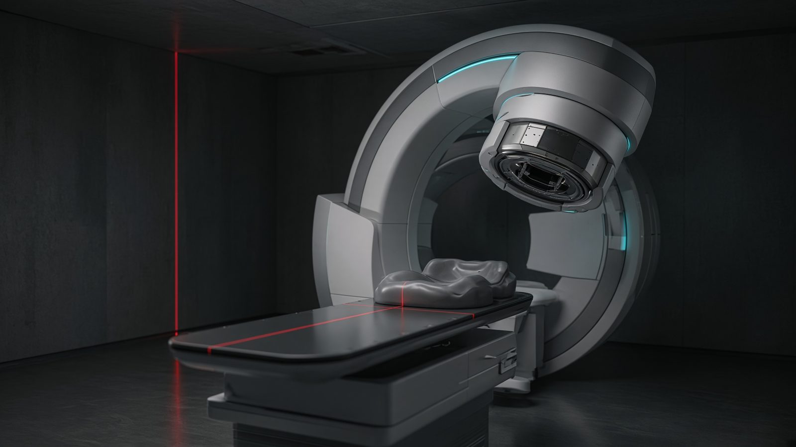
Isocenter
In the treated volume — tumour and OARs at isocenter, after the dose has been delivered.
Open this machineFormula
Typical values
Variables
Results
TD50(v)
Partial-volume TD50
64.9802Gy
t
Probit variable
-2.9907
NTCP
Complication probability
0.0014
NTCP
NTCP
0.14%
Curve
Explanation
What it means
LKB is the classic normal-tissue complication model. TD₅₀ is the uniform whole-organ dose that causes 50% complications, m is the slope (smaller m = steeper), and n is the volume exponent (n→1 parallel organ, n→0 serial). A partial volume v is converted to an equivalent whole-organ dose via the power law, then a probit Φ(t) gives NTCP. Modern practice often prefers gEUD + a logistic, but LKB parameters are still widely published (QUANTEC). This is a working relation in Radiobiology.
Where it is used
Clinically it sits on the Linear accelerator — Isocenter. In the treated volume — tumour and OARs at isocenter, after the dose has been delivered. Radiobiology sits between the prescription and the organ-at-risk: LQ, BED, EQD2, and why 2 Gy is not 2 Gy if the fraction size changed. Use it to compare regimens, not to invent one.
Linear accelerator · Open this machineHow to use it
Enter dose D (Gy), volume fraction v, TD₅₀, m and n from a published fit. Parotid xerostomia: TD₅₀≈40 Gy, n≈0.7, m≈0.18. Cord: n≈0.05, TD₅₀≈67 Gy, m≈0.18. Read t and NTCP. Change one input and watch the curve and the simulation follow.
Symbols
- DDose30 Gy
- vVolume fraction0.5
- TD_50Whole-organ TD5040 Gy
- mSlope0.18
- nVolume exponent0.7
Worked example
A typical case from the default values: D = 30 Gy (Dose); v = 0.5 (Volume fraction); TD_50 = 40 Gy (Whole-organ TD50); m = 0.18 (Slope); n = 0.7 (Volume exponent). Substituting into the relation gives TD50(v) = 64.9802 Gy; t = -2.9907; NTCP = 0.0014; NTCP = 0.14 %. These are teaching numbers — align them with your machine.
Typical values give
- TD50(v) = 64.9802Gy
- t = -2.9907
- NTCP = 0.0014
- NTCP = 0.14%
Where it comes from
The displayed formula is the working relation. t = (D − TD₅₀(v)) / (m TD₅₀(v)), TD₅₀(v) = TD₅₀ / v^n, NTCP = Φ(t). Usual reference: Lyman 1985 / Kutcher & Burman 1989. Derive it in the specialty lesson, then return here to pin the numbers.
Reference: Lyman 1985 / Kutcher & Burman 1989
Assumptions & limits
Uniform dose to fraction v, rest spared. A real DVH needs Kutcher’s effective-volume reduction (v_eff = Σ v_i (D_i/Dmax)^{1/n}) before this formula. Population model — not a prediction for one named patient. Endpoints and fractionation must match the fitted parameters (usually 2 Gy/fx).
Pitfalls
α/β is a model parameter, not a measured organ. BED from incomplete repair or a changed overall time is not the simple n·d·(1+d/(α/β)). Never EQD2 a stereotactic dose with an α/β you did not state. Uniform dose to fraction v, rest spared. A real DVH needs Kutcher’s effective-volume reduction (v_eff = Σ v_i (D_i/Dmax)^{1/n}) before this formula. Population model — not a prediction for one named patient. Endpoints and fractionation must match the fitted parameters (usually 2 Gy/fx).
Keep this
Always write α/β and the fraction size next to a BED or EQD2. Uniform dose to fraction v, rest spared. A real DVH needs Kutcher’s effective-volume reduction (v_eff = Σ v_i (D_i/Dmax)^{1/n}) before this formula. Population model — not a prediction for one named patient. Endpoints and fractionation must match the fitted parameters (usually 2 Gy/fx).
In this specialty