08 Ultrasound
Spatial pulse length and duty factor
SPL = n λ, PD = n/f, DF = PD × PRF.
Listen
Listen · English
Simulation
Spatial pulse length and duty factor — Change the numbers; the scene follows.
Where it works
Ultrasound
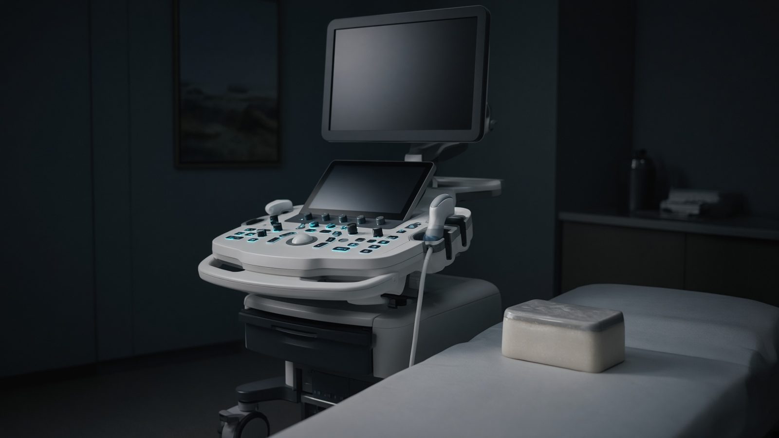
Transducer
At the transducer face — wavelength, pulse length, and the near/far field of the beam.
Open this machineFormula
Variables
Results
SPL
Spatial pulse length
0.924mm
PD
Pulse duration
0.6µs
DF
Duty factor
0.0024
DF
Duty factor
0.24%
Explanation
What it means
Spatial pulse length SPL = n λ, pulse duration PD = n/f, and duty factor DF = PD × PRF. Diagnostic imaging DF is << 1% (the probe listens most of the time); CW Doppler DF = 1. Thermal index scales with DF and output power. This is a working relation in Ultrasound.
Where it is used
Clinically it sits on the Ultrasound — Transducer. At the transducer face — wavelength, pulse length, and the near/far field of the beam. Ultrasound equations sit on the probe face and along the beam: impedance, Snell, Doppler, MI and TI. They explain why gel matters, why aliasing appears, and why a mechanical index is on the screen.
Ultrasound · Open this machineHow to use it
3 cycles at 5 MHz → PD = 0.6 µs. At PRF 4 kHz, DF = 0.24%. Axial resolution ≈ SPL/2 (see that calculator). Change one input and watch the curve and the simulation follow.
Symbols
- nCycles per pulse3
- fFrequency5 MHz
- PRFPulse repetition frequency4 kHz
- cSpeed of sound1,540 m/s
Worked example
A typical case from the default values: n = 3 (Cycles per pulse); f = 5 MHz (Frequency); PRF = 4 kHz (Pulse repetition frequency); c = 1,540 m/s (Speed of sound). Substituting into the relation gives SPL = 0.924 mm; PD = 0.6 µs; DF = 0.0024; DF = 0.24 %. These are teaching numbers — align them with your machine.
Typical values give
- SPL = 0.924mm
- PD = 0.6µs
- DF = 0.0024
- DF = 0.24%
Where it comes from
The displayed formula is the working relation. SPL = n λ, PD = n/f, DF = PD × PRF. Usual reference: Edelman. Derive it in the specialty lesson, then return here to pin the numbers.
Reference: Edelman
Assumptions & limits
Rectangular pulse of n cycles. Real pulses have a smooth envelope so effective n is not integer. MI/TI on the machine include this plus derating.
Pitfalls
Soft-tissue 1540 m/s is an assumption — not a measurement in that patient. Doppler angle 90° gives no shift. MI and TI are on-screen estimates, not absorbed dose. Rectangular pulse of n cycles. Real pulses have a smooth envelope so effective n is not integer. MI/TI on the machine include this plus derating.
Keep this
Gel, angle, and assumed speed of sound — get those three right before you trust a centimetre. Rectangular pulse of n cycles. Real pulses have a smooth envelope so effective n is not integer. MI/TI on the machine include this plus derating.
In this specialty